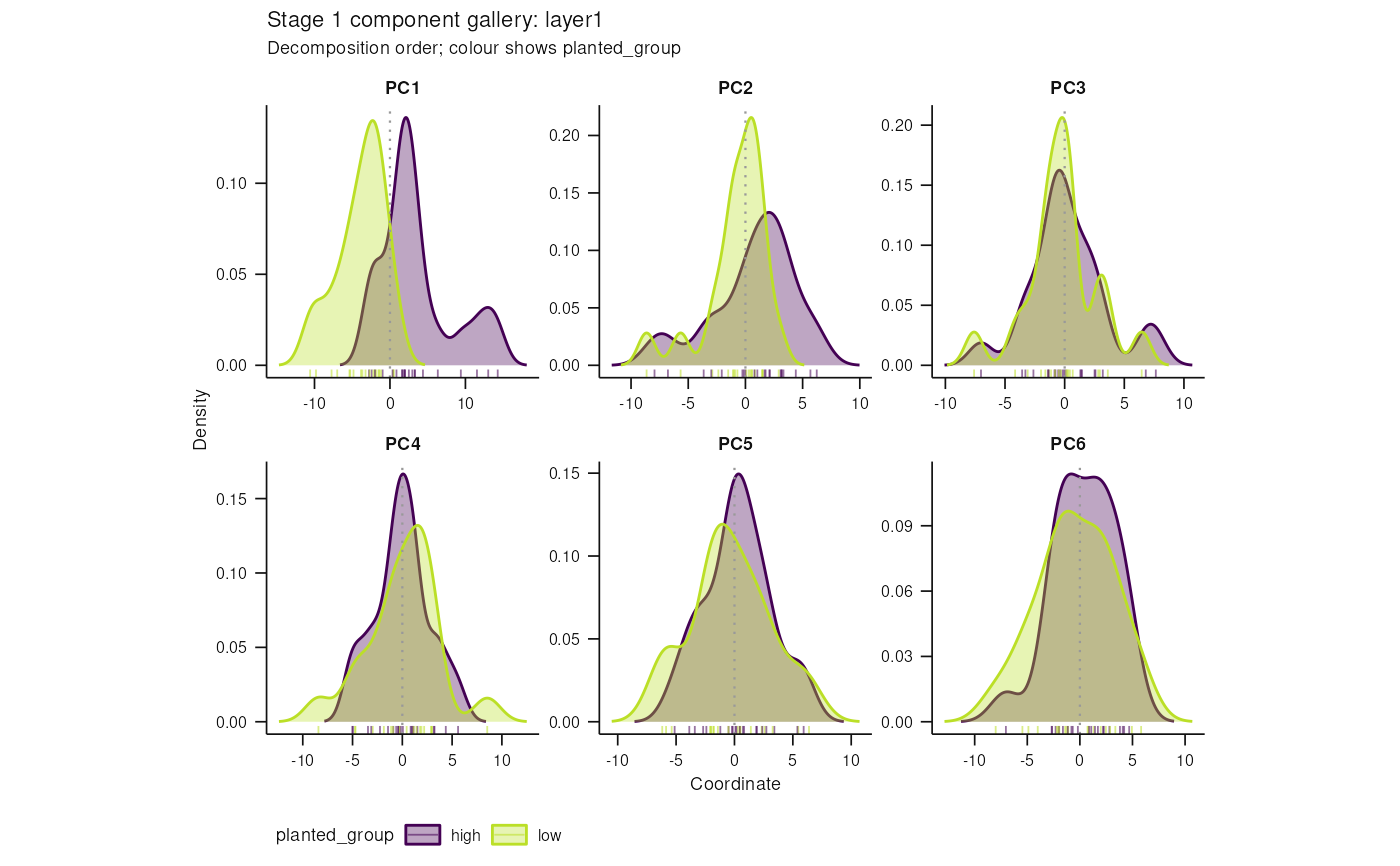
Component gallery coloured by canonically aligned sample metadata

Shows the sample-coordinate distribution for each of the first n_components components as stored density and rug panels in decomposition order. Metadata are read from MAE-level colData and aligned to the selected assay through its canonical sampleMap; row position is never treated as sample identity.

Usage

plot_components(std, colour_by = NULL, n_components = 6L, layer = 1L)

Arguments

std: StateTransitionData with metadata()$stage1 present
colour_by: optional single MAE-level colData column name. Categorical and continuous fields are supported.
n_components: integer number of components to show (default 6)
layer: integer selected assay layer (default 1)

Value

a ggplot object faceted over components in decomposition order

Details

Categorical and continuous metadata colour the rugs while retaining the stored overall density. The gallery does not calculate association scores or rank components; those responsibilities belong to the metadata atlas and proposal workflow.

Examples

std <- synthetic_control(n = 40L, p = 500L, K = 2L, signal = 30, seed = 1L)
ctor <- get_strategy("Decomposer", "hogsvd_averaged")
std2 <- suppressWarnings(decompose(ctor(), std))@value
plot_components(std2, colour_by = "planted_group")