This is a living implementation record, not the package schedule or an acceptance-evidence report. The root ROADMAP is the single scheduling authority. This article shows current user-visible behavior and links to implementation/evidence records. Acceptance evidence is published only from immutable, hash-verified benchmark artifacts.
Current implementation status
| Stage | Name | Status |
|---|---|---|
| Architecture | S4 contracts, registry, container, provenance | ✅ Implemented and CI-tested |
| 0 | Synthetic controls (K=1/K≥2 subspace, exact-stationary double well) | ⚠️ Calibration controls implemented; frozen K=1 recovery/negative-control ladder remains #51 |
| 1 | Single-omic-layer registered SVD | ⚠️ Implemented and visually demonstrated; scientific acceptance remains blocked by #51 and #67 |
| 1 | Comparative decomposition — legacy equal-feature strategies | ⚠️ Implemented; not evidence for heterogeneous multi-omic fitting |
| 1 | Heterogeneous C1/C2 prototype and frozen comparison protocol | ⚠️ Full synthetic run complete; C2 won calibration but failed frozen holdout, so no baseline is accepted and #24 remains blocked |
| 1+ | Descriptive component gallery and legacy project_into()
workflow |
⚠️ Gallery is implemented with canonical metadata alignment; projection remains blocked on #24 |
| 2 | KDE log-density inversion and constrained polynomial smooth | ⚠️ Implemented; ADR 0002 remains provisional-accepted |
Future sequencing, dependencies, and parked capabilities are maintained only in ROADMAP.md, so this article does not duplicate a second planned-work list.
Transient benchmark workspaces
Stage 1 benchmark helpers place their checkpoint workspaces under the
repository .scratch/ directory by default. Set
options(landscapeR.scratch_root = "/path/to/scratch")
before calling a benchmark helper when transient state should live on
another local or HPC filesystem. An explicit workspace
argument still takes precedence.
Biological instantiations
| Dataset | Modality | Status |
|---|---|---|
| AML/CML (Cbfb-MYH11, BCR-ABL) | mRNA, miRNA | Historical exploratory context only; raw data are not in this repository and no claim is current |
| Pogona TSD | mRNA | Planned only; requires a validated geometry/applicability assessment |
| Islet/diabetes multi-omic | mRNA + ATAC + genotype | Planned only; rank-deficient genotype layer is a required Stage 1 stress case |
Analysis intent lifecycle (AnalysisSpecification v2)
A component decision now resolves rather than replaces its target. Every specification retains the target field and its neutral contrast/order/direction; confirmation adds the frozen-basis component and analyst decision provenance.
proposal_id <- strrep("a", 64L)

spec_draft <- analysis_specification(
  id = "condition-axis",
  target_field = "condition",
  target_type = "binary",
  reference_level = "control",
  comparison_level = "disease"
)

spec_proposal <- analysis_specification(
  id = "condition-axis",
  target_field = "condition",
  target_type = "binary",
  reference_level = "control",
  comparison_level = "disease",
  lifecycle = "proposal",
  proposal_digest = proposal_id
)

spec_confirmed <- analysis_specification(
  id = "condition-axis",
  target_field = "condition",
  target_type = "binary",
  reference_level = "control",
  comparison_level = "disease",
  lifecycle = "confirmed",
  selected_component = 2L,
  proposal_digest = proposal_id,
  proposal_decision = "accepted",
  analyst_rationale = "Accepted the predeclared top-ranked target axis."
)

data.frame(
  lifecycle = c(spec_draft@lifecycle,
                spec_proposal@lifecycle,
                spec_confirmed@lifecycle),
  target = rep("control -> disease", 3L),
  proposal = c("absent", "present", "retained"),
  selected_component = c(NA_integer_, NA_integer_,
                         spec_confirmed@selected_component),
  decision = c("absent", "absent", spec_confirmed@proposal_decision)
)
#>   lifecycle             target proposal selected_component decision
#> 1     draft control -> disease   absent                 NA   absent
#> 2  proposal control -> disease  present                 NA   absent
#> 3 confirmed control -> disease retained                  2 accepted
Legacy v1 objects migrate only through
migrate_analysis_specification(). Target-only v1 objects
require explicit direction; component-only v1 objects also require the
missing target and proposal decision record. Migration fails rather than
inventing intent or dropping the legacy component. See the complete
v2 and migration contract.
Stage 0 — Synthetic validation
The pipeline is tested against two synthetic ground truths.
Every successful Stage 0 generator records its complete generator
parameters, seed, and explicit claim status in provenance. Invalid
potential controls raise a typed validation error before they can become
evidence. A control_ladder() sweep retains failures as rows
instead of discarding the rest of the grid. The small proof below
requests one supported two-layer cell and one unsupported single-layer
cell from the legacy HO-GSVD adapter.
| n | p | K | signal | status | failure_class | reason | requested_cells | completed_cells | failed_cells |
|---|---|---|---|---|---|---|---|---|---|
| 8 | 8 | 2 | 20 | success | 2 | 1 | 1 | ||
| 8 | 8 | 1 | 20 | failure | StageResult | hogsvd_averaged requires at least 2 omic layers | 2 | 1 | 1 |
The table also carries requested, completed, and failed cell totals. This is an implementation and calibration-input integrity contract, not evidence that a decomposition strategy is scientifically accepted.
Two-group control
synthetic_control() generates two groups of samples with
a planted signal on the first component. Used to verify Stage 1 recovers
the correct axis.
library(landscapeR)

std <- synthetic_control(n = 40L, p = 500L, K = 2L, signal = 30, seed = 1L)
ctor <- get_strategy("Decomposer", "hogsvd_averaged")
std1 <- suppressWarnings(decompose(ctor(), std))@value

plot_spectrum(std1)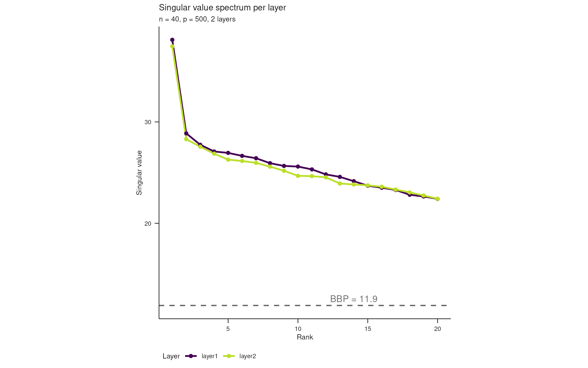
hogsvd_averaged and hogsvd_prereduced are
legacy baseline adapters for two or more layers defined on equal-sized
feature spaces. They do not implement the heterogeneous or
rank-deficient HO-GSVD candidates being evaluated under ADR 0001 and
tracked in #49. Their
input boundary is explicit:
| Input | Outcome |
|---|---|
| Two or more finite numeric layers with identical, unique, ordered feature identifiers | Typed Stage 1 success |
| Fewer than two layers | Typed failure with a reason |
| Different, missing, duplicated, or reordered feature identifiers | Typed unsupported-design failure with a reason |
| Invalid parameters, non-finite values, or numerical failure | Typed failure with a reason |
These outcomes describe implementation safety only. They do not constitute scientific acceptance of either legacy strategy.
The component gallery aligns MAE-level metadata through each assay’s canonical sample map. Categorical metadata colour stored group-specific densities and rugs; continuous metadata colour rugs beneath the stored overall density, so rendering never refits a descriptive smoother. When a component or categorical group has insufficient numerical spread for kernel-density estimation, its sample coordinates remain visible as rugs and the separate scientific caption identifies the unavailable density slice.
plot_components(
  std1,
  colour_by = "planted_group",
  n_components = 4L
)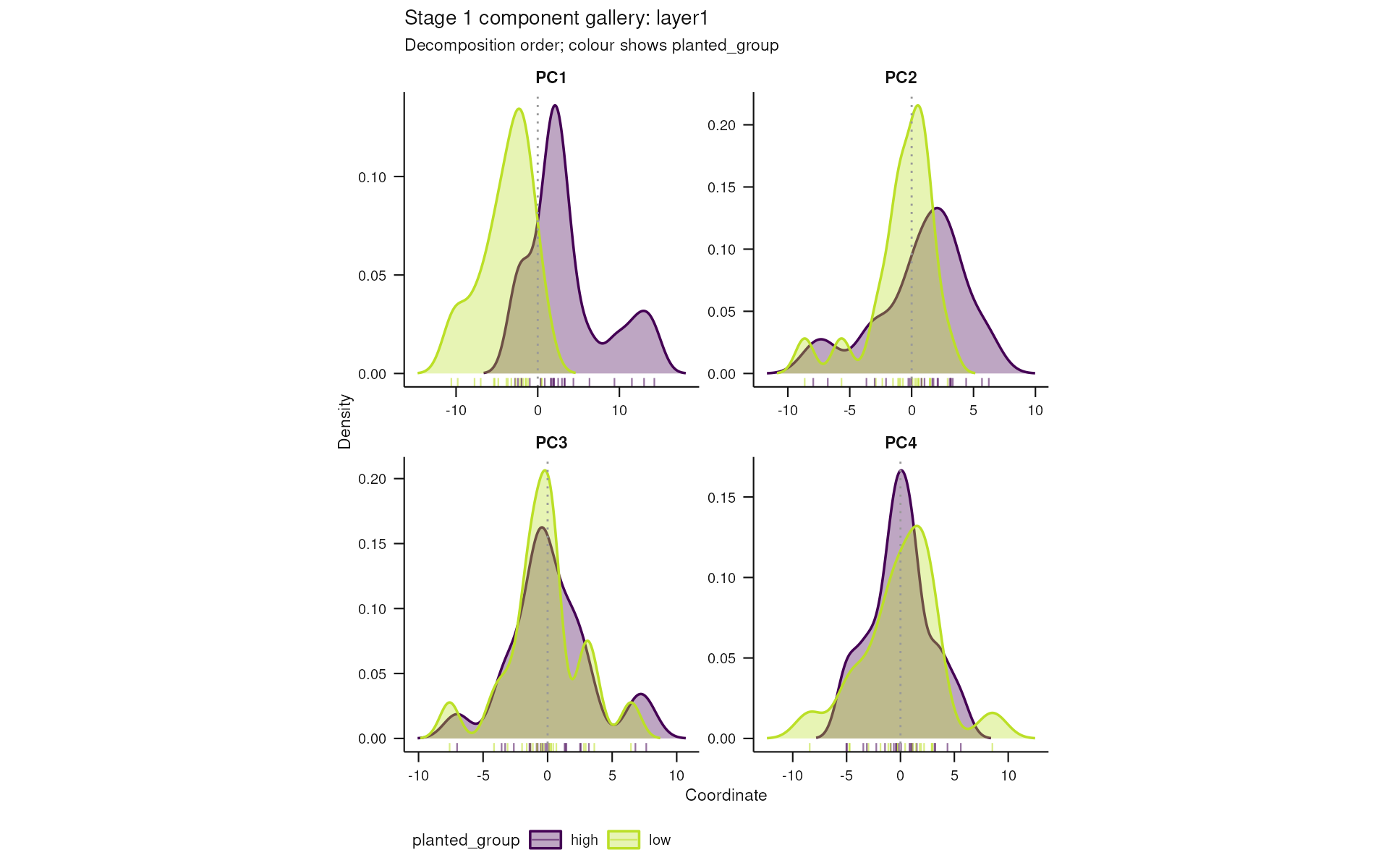
Categorical descriptive gallery: planted synthetic groups colour densities and rugs after canonical sample alignment.
plot_components(
  std1,
  colour_by = "u_shared",
  n_components = 4L
)
#> Ignoring unknown labels:
#> • fill : "u_shared"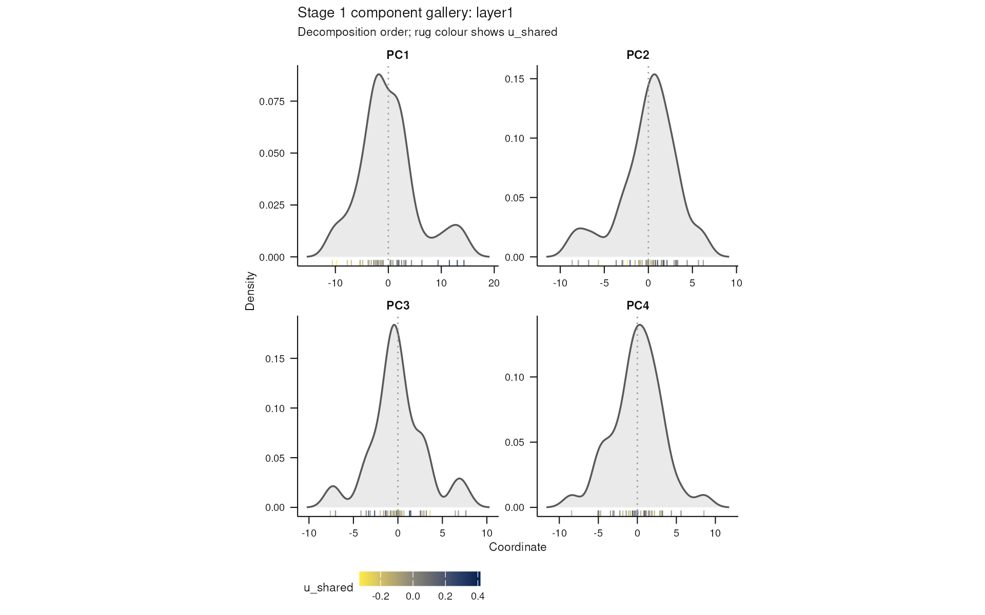
Continuous descriptive gallery: the planted continuous coordinate colours the rug while the overall component density remains visible.
Cold-reader conclusion: metadata colour is visible for both categorical and continuous fields, panels remain in decomposition order, and the gallery makes no association score or component recommendation. Scientific ranking and analyst confirmation remain the responsibility of the future atlas/proposal workflow.
K=1 single-omic-layer SVD and double-well calibration (#50)
Before issue #50, the only runnable development-log path duplicated a single-omic-layer coordinate assay so it could enter a K≥2 HO-GSVD strategy. That workaround obscured the actual capability boundary and recorded the wrong strategy for a K=1 analysis.
| Condition | Before #50 | After #50 |
|---|---|---|
| K=1 synthetic subspace | Rejected by the generator | First-class control with planted subspace truth |
| Stage 1 strategy | Duplicate the assay and call HO-GSVD | Registered exactly-one-omic-layer svd
|
| Double-well observations | Thinned trajectory in the older estimator-level control | Independent exact-stationary draws for the K=1 end-to-end calibration control |
| Evidence status | Ambiguous development workaround | Explicitly non_evidentiary_calibration
|
The current development path now keeps K=1 explicit from generation through Stage 1 and the cross-sectional Stage 2 estimator:
std_k1 <- synthetic_k1_double_well_control(
  n = 200L, p = 100L, noise_sd = 0.03, seed = 50L
)

svd_ctor <- get_strategy("Decomposer", "svd")
std_k1_s1 <- suppressWarnings(decompose(svd_ctor(), std_k1))@value

coordinate_k1 <- colData(std_k1)$x_coord

empirical_density <- ggplot2::ggplot(
  data.frame(coordinate = coordinate_k1),
  ggplot2::aes(x = coordinate)
) +
  ggplot2::geom_density(fill = "#67A9CF", alpha = 0.45, linewidth = 0.8) +
  ggplot2::geom_rug(alpha = 0.35) +
  ggplot2::labs(
    title = "Descriptive evidence: planted cross-sectional coordinate density",
    x = "State-transition coordinate",
    y = "Density"
  ) +
  ggplot2::theme_bw(base_size = 11)
print(empirical_density)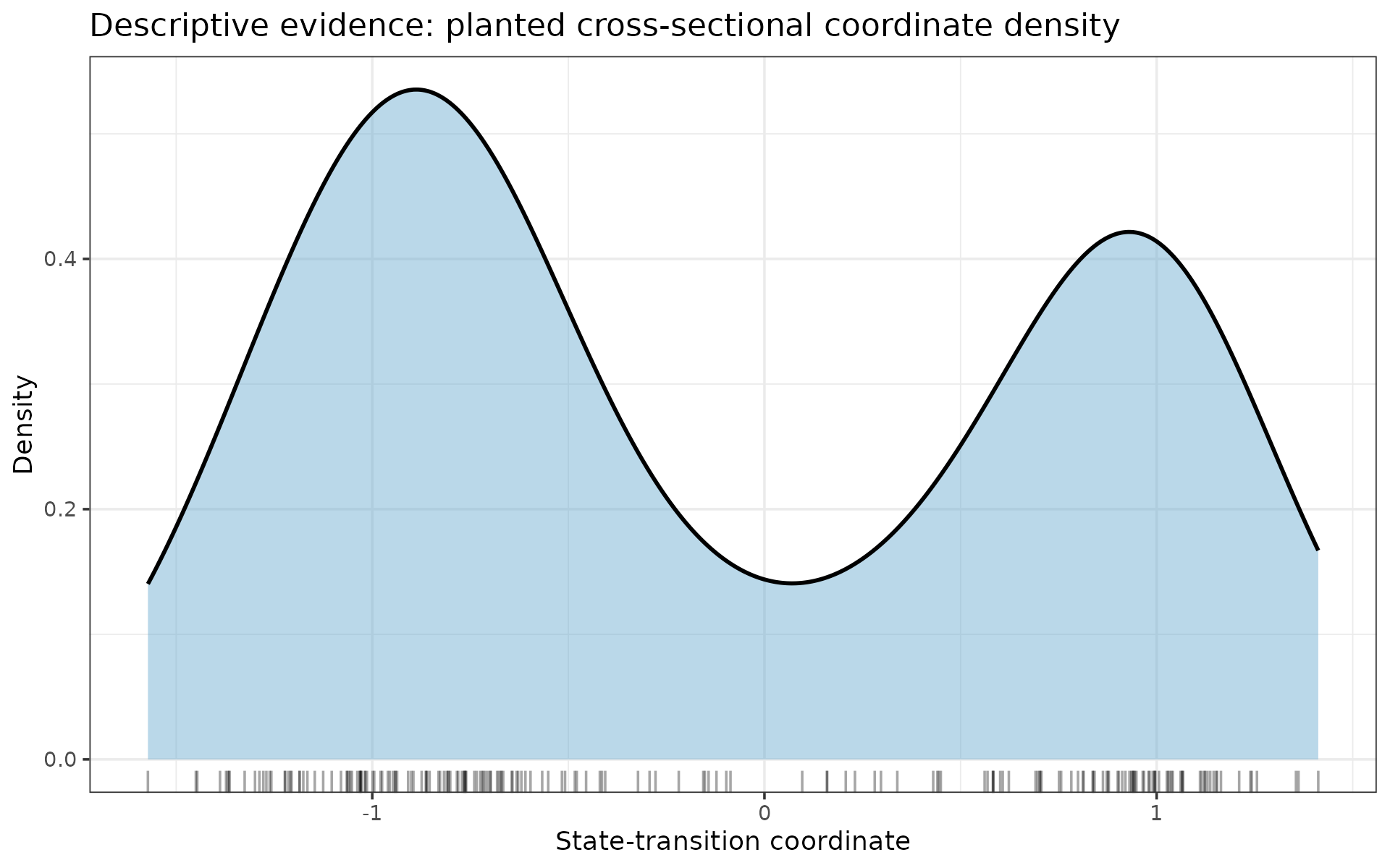
Descriptive evidence: empirical density of the planted cross-sectional coordinate supplied to the single-omic-layer expression control.
dynamics_ctor <- get_strategy("DynamicsEstimator", "kde_logdensity")
std_k1_s2 <- estimate_dynamics(dynamics_ctor(), std_k1_s1)@value
plot_potential(std_k1_s2, show_critical_points = FALSE) +
  ggplot2::labs(
    subtitle = paste(
      "Critical-point classification omitted — uncertainty is not yet",
      "estimated; calibration-only output"
    )
  )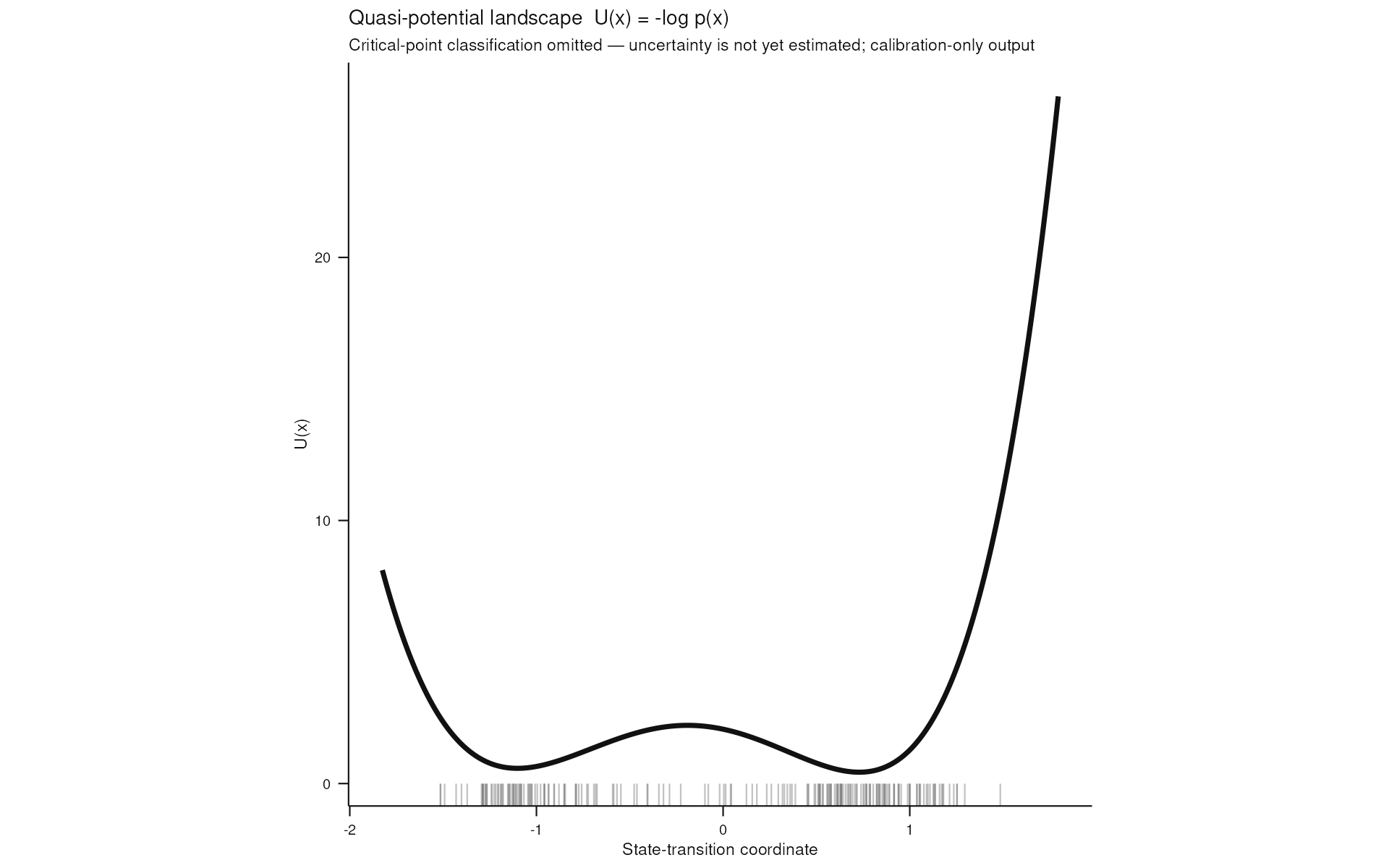
Hypothesis-conditioned interpretation: the fitted calibration-only quasi-potential; critical-point classification is deliberately omitted because uncertainty is not yet estimated.
Cold-reader conclusion: the single-omic-layer expression control now passes through the registered SVD strategy and produces the expected two-well quasi-potential without fabricating a second omic layer. The public synthetic input distribution remains visible before the fitted interpretation, and the plot omits critical-point classification because uncertainty is not yet estimated.
This is implementation and calibration proof, not acceptance evidence. The frozen K=1 thinness, negative-control, and independent acceptance protocol is tracked in #51; the AML-grounded target/confounder control is #67.
k1_calibration <- suppressWarnings(k1_double_well_calibration(
  n = 200L, p = 100L, noise_sd = 0.03, seed = 50L
))

knitr::kable(data.frame(
  diagnostic = c(
    "Evidence status",
    "Stage 1 strategy",
    "Subspace angle (degrees)",
    "Mean well-location error",
    "Barrier-location error",
    "Barrier-height error"
  ),
  value = c(
    k1_calibration$evidence_status,
    k1_calibration$decomposer,
    format(round(k1_calibration$subspace_angle_deg, 3), nsmall = 3),
    format(round(k1_calibration$well_error, 3), nsmall = 3),
    format(round(k1_calibration$barrier_error, 3), nsmall = 3),
    format(round(k1_calibration$barrier_height_error, 3), nsmall = 3)
  )
), col.names = c("Diagnostic", "Observed calibration output"))| Diagnostic | Observed calibration output |
|---|---|
| Evidence status | non_evidentiary_calibration |
| Stage 1 strategy | svd |
| Subspace angle (degrees) | 1.431 |
| Mean well-location error | 0.084 |
| Barrier-location error | 0.050 |
| Barrier-height error | 0.220 |
The table deliberately contains no pass, acceptance, or eligibility judgement. Those decisions belong to the frozen independent protocol, not this disclosed calibration run.
Declared KDE bandwidth
Stage 2 treats bandwidth as part of the estimator specification
rather than a hidden fitting choice. The registered default remains
ks::hpi(). A finite positive numeric value can instead be
declared for a Stage 0 sweep; the method and resolved value are stored
with the fitted result and its provenance.
default_kde <- estimate_dynamics(dynamics_ctor(), std_k1_s1)
explicit_kde <- estimate_dynamics(
  dynamics_ctor(params = list(
    bandwidth_method = "explicit",
    bandwidth_value = 0.25
  )),
  std_k1_s1
)

default_stage2 <- metadata(default_kde@value)$stage2
explicit_stage2 <- metadata(explicit_kde@value)$stage2
default_bandwidth_label <- sprintf(
  "Default hpi (h = %.3f)",
  default_stage2$bandwidth_value
)
bandwidth_curves <- rbind(
  data.frame(
    coordinate = default_stage2$x,
    quasi_potential = default_stage2$U - min(default_stage2$U),
    estimator = default_bandwidth_label
  ),
  data.frame(
    coordinate = explicit_stage2$x,
    quasi_potential = explicit_stage2$U - min(explicit_stage2$U),
    estimator = "Explicit (h = 0.250)"
  )
)

ggplot2::ggplot(
  bandwidth_curves,
  ggplot2::aes(x = coordinate, y = quasi_potential, colour = estimator)
) +
  ggplot2::geom_line(linewidth = 0.8) +
  scale_colour_landscapeR(
    "binary",
    reference_level = default_bandwidth_label,
    focal_level = "Explicit (h = 0.250)"
  ) +
  ggplot2::labs(
    x = "State-transition coordinate",
    y = "Relative quasi-potential",
    colour = "Bandwidth"
  ) +
  ggplot2::guides(colour = ggplot2::guide_legend(ncol = 1L)) +
  theme_landscapeR(base_size = 11) +
  ggplot2::theme(legend.position = "bottom")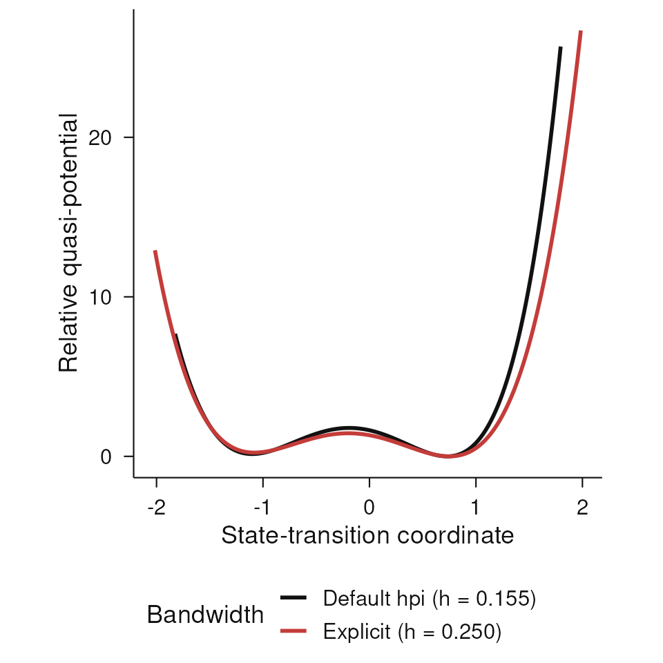
Default and explicitly declared bandwidths applied to the same frozen
synthetic cross-sectional coordinate. Black shows the registered
ks::hpi() estimator (resolved bandwidth printed in the
legend); red shows the illustrative explicit value 0.25. Curves are
shifted to a minimum of zero so their shapes can be compared without
implying an absolute potential origin. This is implementation proof that
bandwidth is sweepable and provenance-recorded; neither setting is
accepted for biological inference from this visual comparison.
degenerate_kde <- std_k1_s1
degenerate_stage1 <- metadata(degenerate_kde)$stage1
degenerate_stage1@coords_k <- lapply(
  degenerate_stage1@coords_k,
  function(coords) matrix(1, nrow = nrow(coords), ncol = ncol(coords))
)
degenerate_metadata <- metadata(degenerate_kde)
degenerate_metadata$stage1 <- degenerate_stage1
metadata(degenerate_kde) <- degenerate_metadata
degenerate_result <- estimate_dynamics(dynamics_ctor(), degenerate_kde)

knitr::kable(data.frame(
  outcome = degenerate_result@status,
  diagnostic = degenerate_result@reason
), col.names = c("Typed outcome", "Stable diagnostic"))| Typed outcome | Stable diagnostic |
|---|---|
| failure | estimate_dynamics: coordinate support must contain at least two distinct finite values with a finite positive range. |
The degenerate coordinate is rejected before an external bandwidth or
density fit is attempted. Backend failures are likewise returned as
typed Stage 2 failures, so a sweep can retain the failed cell without
converting an external ks exception into a pipeline
crash.
Historical AML/CML exploratory context
Earlier exploratory work used AML/CML cohorts as a translation target
for the Rockne–Frankhouser literature. The raw matrices and generated
local preprocessing objects are deliberately not
included in this public repository, so the old AML chunks are removed
rather than presented as runnable analysis. A minimal mapping of
already-public mouse sample identifiers to the checksum-pinned
authoritative sample_weeks values is included solely to
make data lineage testable.
The corrected GSE133642 preparation keeps the source-study roles distinct from landscapeR’s use of both matrices as real biological validation data:
| Prepared layer | Source-study role | Observations | landscapeR role |
|---|---|---|---|
mrna_primary_2018 |
2018 training cohort | 132 | future exploratory discovery basis |
mrna_supp_2016 |
2016 validation cohort 1 | 101 | later hostile batch/time-confounded projection test |
Its longitudinal declaration names only mouse_id and
exact numeric sample_weeks (unit: weeks). Categorical
labels are inert, and no endpoint or event semantics are inferred.
These data are not evidence for the package’s present claims. Under the evidence-first validation plan, real-data Stage 2 inference is blocked until the frozen generic Stage 0 ladder has passed, ADR 0002 has finalized thresholds, and a separate applicability and confirmation workflow has been specified. Any future AML/CML article will include a public data manifest, a fixed analysis specification, and the required confirmation/claim-status diagnostics.
Evidence status
The accepted Stage 1 v2 protocol compared two prototype estimators on
synthetic, heterogeneous-feature controls. Its completed, hash-verified
full artifact selected C2_block_scaled_svd in calibration,
but C2 failed the frozen holdout acceptance thresholds. Consequently no
Stage 1 baseline is accepted and #24 remains blocked. The Stage 1 synthetic evidence article
renders the immutable artifact; neither C1 substitution nor C2 tuning is
permitted from the consumed v2 holdout.
Similarly, the Stage 2 implementation is an auditable estimator, not yet a validated biological inference engine. See ADR 0002 and the Stage 0 protocol for its current claim boundary.
Architecture notes
The package uses a contract/registry pattern — all
stage algorithms are S4 virtual classes with generics
(decompose, estimate_dynamics). Concrete
strategies are registered by name and retrieved at runtime:
list_strategies("Decomposer")
#> [1] "Decomposer:hogsvd_averaged"   "Decomposer:hogsvd_prereduced"
#> [3] "Decomposer:svd"
list_strategies("DynamicsEstimator")
#> [1] "DynamicsEstimator:kde_logdensity"
This means adding a new algorithm (e.g. Kempf HO-GSVD, neural SDE) is
a register_strategy() call with no changes to calling code
or tests.
Implementation index
- 2026-07-14 — K=1 foundation and visual landing-proof policy: #50 adds the registered single-omic-layer SVD and calibration control; #68 makes the pull request the canonical visual transition record. The full before/after proof is co-located with the diff in PR #69. This remains implementation work, not K=1 acceptance evidence.
Last updated: 2026-07-14. Documentation site: https://drejom.github.io/landscapeR/.